What is Storchastic?¶

On this page we introduce the ideas behind Storchastic before diving into the code, and explain what kinds of problems it could be applied to. If you are already familiar with stochastic computation graphs [A12] and gradient estimation, you can safely skip this page and start at Sampling, Inference and Variance Reduction.

Stochastic computation graphs¶

PyTorch relies on computation graphs for its automatic differentiation algorithm. These graphs keeps track of all operations that happen while executing PyTorch code by recording the inputs and outputs to PyTorch functions. Each node represents the output of some function. Consider the differentiable function

\[f=(a + b) \cdot (b + c)^2\]

This function can be represented using a (deterministic) computation graph as

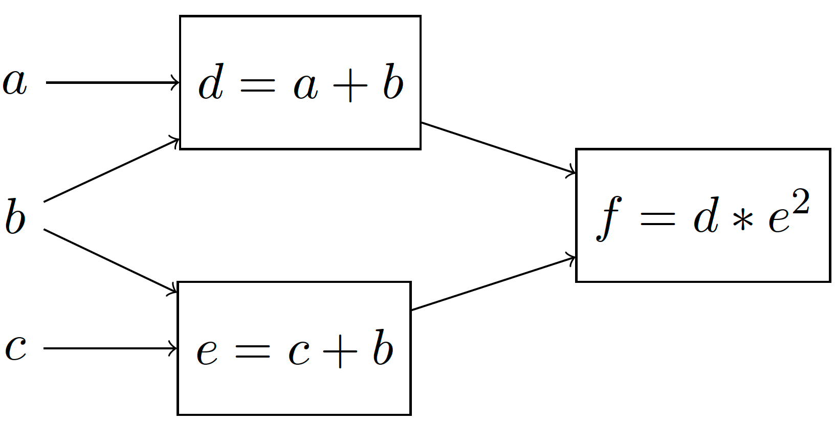
An example of a deterministic computation graph.

By assigning to \(a, b, c\) a concrete value, we can deterministically compute the value of \(f\). PyTorch then uses reverse-mode differentiation on such graphs to find the derivatives with respect to the parameters.

However, in many applications we are interested in computation graphs with stochastic nodes. Stochastic nodes are when we take a sample from a distribution, and use the resulting sample to compute the output. For example, suppose that we sample \(e\) from a normal distribution with mean c+b and standard deviation 1. We can represent this using a stochastic computation graph:

An example of a stochastic computation graph.

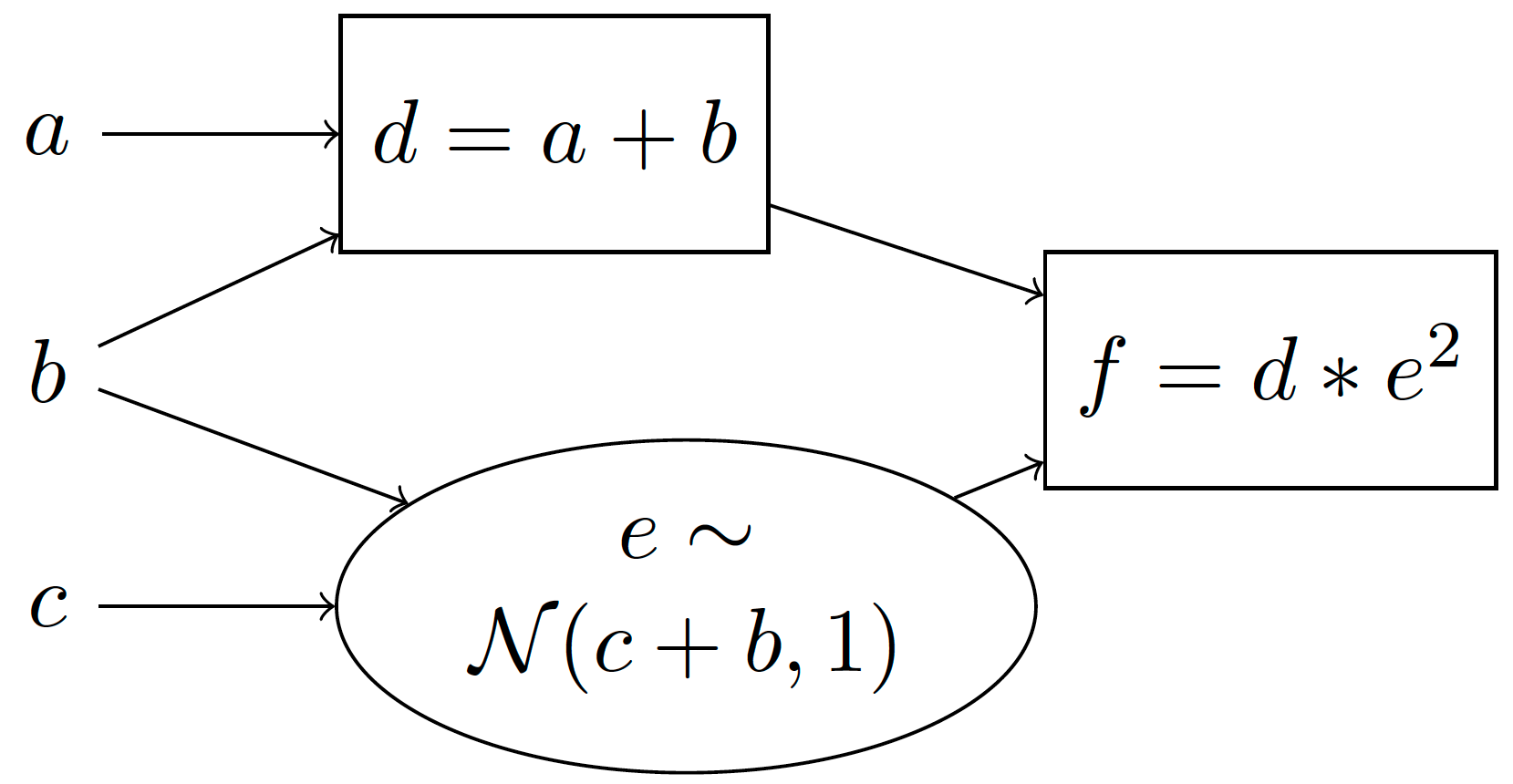
We use rectangles to denote deterministic computations and ellipses to denote stochastic computations. We can also equivalently represent this using a generative story:

Compute \(d=a+b\)
Sample \(e\sim \mathcal{N}(c+b, 1)\) 1
Compute \(f=d\cdot e^2\)

A generative story is a nice and easy to understand way to show how outputs are generated step-by-step. The goal of Storchastic is to be able to write code that looks just like a generative story. Because of this, we will present both stochastic computation graphs and their associated generative stories in these tutorials.

A very common question in stochastic computation graphs is: What is the expected value of \(f\)? Mathematically, this is computed as:

\[\mathbb{E}_{e\sim \mathcal{N}(c+b, 1)}[(a+b)\cdot e^2]=\int p(e|b, c)\cdot (a+b)\cdot e^2\ de\]

This expression requires computing the integral over all values of \(e\), which is generally intractable. 2 A very common method to approximate expectations is to use Monte Carlo methods: Take some (say \(S\)) samples of \(e\) from the normal distribution and average out the resulting values of \(f\):

(1)¶\[\mathbb{E}_{e\sim \mathcal{N}(c+b, 1)}[(a+b)\cdot e^2]\approx \frac{1}{S}\sum_{i=1}^S (a+b)\cdot e_i^2, \quad e_1, ..., e_S\sim \mathcal{N}(c+b, 1)\]

Gradient estimation¶

We have shown a simple model with a stochastic node, and we have shown how to compute samples of the output. Next, assume we are interested in the derivative with respect to input \(c\) \(\frac{\partial}{\partial c}\mathbb{E}_{e\sim \mathcal{N}(c+b, 1)}[(a+b)\cdot e^2]\). For the same reason as before, we will use Monte Carlo estimation and sample some values from the distribution to estimate the derivatives.

There is however a big issue here: Sampling is not a differentiable procedure! An easy way to see this is by looking at equation (1): \(c\) does not appear in the Monte Carlo estimation. This means we cannot use reverse-mode differentiation to compute the derivatives with respect to the inputs \(b,c\). Luckily, we can use gradient estimation methods [A11].

The pathwise derivative¶

A well known gradient estimation method is the pathwise derivative [A3] which is commonly referred to in Machine Learning as reparameterization [A6]. We explain this estimation method by transforming the previous stochastic computation graph to one that is equivalent:

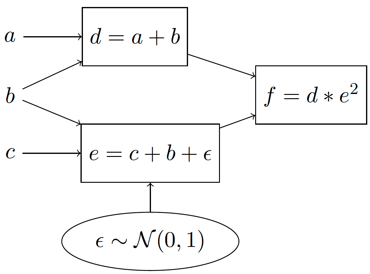
Which has the following generative story:

Compute \(d=a+b\)
Sample \(\epsilon \sim \mathcal{N}(0, 1)\)
Compute \(e = c+b + \epsilon\)
Compute \(f=d*e^2\).

The idea behind the pathwise derivative is to move the sampling procedure outside of the computation path, so that the derivatives with respect to \(b, c\) can now readily be computed using automatic differentiation! It works because it shifts the mean of the 0-mean normal distribution by \(c+b\).

Unfortunately, this does not end our story, because the pathwise derivative has two heavy assumptions that limit its applicability. The first is that a reparameterization must exist for the distribution to sample from. For the normal distribution, this reparameterization is very simple, and a reparameterization has been derived for many other useful continuous distributions. However, no (unbiased 3 ) reparameterization exists for discrete distributions! Secondly, the pathwise derivative requires there to be a differentiable path from the sampling step to the output. In many applications, such as in Reinforcement Learning, this is not the case.

The score function¶

The pathwise derivative is a great choice if it is applicable because it is unbiased and usually has low variance. When it is not applicable, we can turn to the score function, which is known in Reinforcement Learning as REINFORCE. Rewrite \(f\) as a function of \(e\) using \(f(e)=(a+b)\cdot e^2\). Then

\[\begin{split}\frac{\partial}{\partial c}\mathbb{E}_{e\sim \mathcal{N}(c+b, 1)}[f(e)] &= \frac{\partial}{\partial c}\int p(e|b, c)f(e) de \\ &= \int \frac{\partial}{\partial c} p(e|b, c) \frac{p(e|b, c)}{p(e|b, c)}f(e) de \\ &= \int p(e|b, c)f(e) \frac{\partial}{\partial c}\log p(e|b, c) de\\ &= \mathbb{E}_{e\sim \mathcal{N}(c+b, 1)}\left[f(e) \frac{\partial}{\partial c} \log p(e|b, c)\right]\end{split}\]

By introducing the \(\log p(e|b, c)\) term in the expectation, Monte Carlo samples now depend on \(c\) and so we can compute a derivative with respect to \(c\)! Additionally, the score function can be used for any probability distribution and also works for non-differentiable functions \(f\): It is universally applicable!

That sounds too good to be true, and unfortunately, it is. The score function is notorious for having very high variance. The variance of an estimation method can be seen as the average difference between the samples. That means we will need to look at many more samples to get a good idea of what gradient direction to follow.

Luckily, there is a significant amount of literature on variance-reduction methods, that aim to reduce the variance of the score function. These greatly help to apply stochastic computation graphs in practice! Storchastic implements many of these variance-reduction methods, to allow using stochastic computation graphs with non-differentiable functions and discrete distributions.

Applications¶

Next, we show some common applications of gradient estimation to get an idea of what kind of problems Storchastic can be useful for.

Reinforcement Learning¶

In Reinforcement Learning (RL), gradient estimation is a central research topic. The popular policy gradient algorithm is the score function applied to the MDP model that is common in RL:

\[\nabla_\theta J(\theta) \propto \mathbb{E}_{s\sim p_\theta(s), a\sim p_\theta(a|s)}[Q_\pi(s, a)\nabla_\theta \log p_\theta(a|s)]\]

Decreasing the variance of this estimator is a very active research area, as lower-variance estimators generally require fewer samples to train the agent. This is often done using so-called “actor-critic” algorithms, that reduce the variance of the policy gradient estimator using a critic which predicts how good an action is relative to other possible actions. Other recent algorithms employ the pathwise derivative to make use of the gradient of the critic [A4][A9]. There is active work on generalizing these ideas to stochastic computation graphs [A13].

Variational Inference¶

Variational inference is a general method for Bayesian inference. It introduces an approximation to the posterior distribution, then minimizes the distance between this approximation and the actual posterior. In the deep learning era, so-called ‘amortized inference’ is used, where the approximation is a neural network that predicts the parameters of the approximate distribution. To train the parameters of this neural network, samples are taken from the approximate posterior, and gradient estimation is used. For continuous posteriors, the pathwise derivative is usually employed [A6], but for discrete posteriors, the choice of gradient estimator is an active area of research [A5].

Discrete Random Variables¶

Discrete random variables are challenging to deal with in practice, but have many promising applications. Deep learning usually acts in the continuous space and discrete random variables are a theoretically motivated way to do some computation in the discrete world. This allows deep learning methods to make clear cut decisions, instead of a continuous attention vector over all options which does not scale in practice.

For example, a variational autoencoder (VAE) with a discrete latent space could be useful to discern properties on the data. Other applications include querying Wikipedia within a language model [A7], learning how to generate computer programs [A1][A8] and hard attention layers [A2]. Additionally, sequence models such as neural machine translation can be trained directly on BLEU scores using gradient estimation.

Footnotes¶

1: \(\mathcal{N}(\mu, \sigma)\) is a normal distribution with mean \(\mu\) and standard deviation \(\sigma\).
2: For a simple expression like this, a closed-form analytical form can pretty easily be found. However, usually our models are much more complex and non-linear.
3: There is a very popular biased and low-variance reparameterization called the Gumbel-softmax-trick [A5][A10], though!

References¶

A1: Rudy Bunel, Matthew Hausknecht, Jacob Devlin, Rishabh Singh, and Pushmeet Kohli. Leveraging grammar and reinforcement learning for neural program synthesis. arXiv preprint arXiv:1805.04276, 2018.
A2: Yuntian Deng, Yoon Kim, Justin Chiu, Demi Guo, and Alexander Rush. Latent alignment and variational attention. In Advances in Neural Information Processing Systems, 9712–9724. 2018.
A3: Paul Glasserman and Yu-Chi Ho. Gradient estimation via perturbation analysis. Volume 116. Springer Science & Business Media, 1991.
A4: Tuomas Haarnoja, Aurick Zhou, Pieter Abbeel, and Sergey Levine. Soft actor-critic: off-policy maximum entropy deep reinforcement learning with a stochastic actor. arXiv preprint arXiv:1801.01290, 2018.
A5(1,2): Eric Jang, Shixiang Gu, and Ben Poole. Categorical reparameterization with gumbel-softmax. arXiv preprint arXiv:1611.01144, 2016.
A6(1,2): Diederik P Kingma and Max Welling. Auto-encoding variational bayes. arXiv preprint arXiv:1312.6114, 2013.
A7: Patrick Lewis, Ethan Perez, Aleksandara Piktus, Fabio Petroni, Vladimir Karpukhin, Naman Goyal, Heinrich Küttler, Mike Lewis, Wen-tau Yih, Tim Rocktäschel, Sebastian Riedel, and Douwe Kiela. Retrieval-augmented generation for knowledge-intensive nlp tasks. 2020. arXiv:2005.11401.
A8: Chen Liang, Mohammad Norouzi, Jonathan Berant, Quoc V Le, and Ni Lao. Memory augmented policy optimization for program synthesis and semantic parsing. In Advances in Neural Information Processing Systems, 9994–10006. 2018.
A9: Timothy P Lillicrap, Jonathan J Hunt, Alexander Pritzel, Nicolas Heess, Tom Erez, Yuval Tassa, David Silver, and Daan Wierstra. Continuous control with deep reinforcement learning. arXiv preprint arXiv:1509.02971, 2015.
A10: Chris J Maddison, Andriy Mnih, and Yee Whye Teh. The concrete distribution: a continuous relaxation of discrete random variables. arXiv preprint arXiv:1611.00712, 2016.
A11: Shakir Mohamed, Mihaela Rosca, Michael Figurnov, and Andriy Mnih. Monte carlo gradient estimation in machine learning. arXiv preprint arXiv:1906.10652, 2019.
A12: John Schulman, Nicolas Heess, Theophane Weber, and Pieter Abbeel. Gradient estimation using stochastic computation graphs. In Advances in Neural Information Processing Systems. 2015. arXiv:1506.05254.
A13: Théophane Weber, Nicolas Heess, Lars Buesing, and David Silver. Credit assignment techniques in stochastic computation graphs. arXiv preprint arXiv:1901.01761, 2019.